TL;DR: How does this paper change how we model latent variables?

In many political science models, the key predictor is a latent variable (like ideology or democracy) that we only ever observe with error. This paper shows that some popular “corrections” for that uncertainty actually make bias worse, then introduces a simple split‑indicator correction that largely fixes the problem.

• Latent predictors (e.g., ideology, knowledge, democracy indices) are always noisy and live on an arbitrary scale.
• Standard fixes like the method of composition and off‑the‑shelf instrumental variables (IV) can worsen bias instead of reducing it.
• We propose a split‑indicator, correlation‑adjusted estimator that works with additive scores, factor models, or machine learning, without joint modeling.
• Across simulations and real data, corrected effects are often 10–50% larger than naive estimates that ignore measurement error.
• Open‑source software makes the procedure easy to use in applied work.

What are latent variables, and why do they create hidden bias?

In political science, many core concepts are latent: we care about things like political ideology, democratic quality, or political knowledge, but we only see them indirectly through survey answers, expert ratings, or other indicators. Researchers then plug these estimated latent scores into regressions as predictors, which builds measurement error directly into the right‑hand side of the model.

That measurement error has a well‑known consequence: it pushes slope estimates toward zero, a classic problem called attenuation bias. The twist with latent variables is that they also have no natural scale, so researchers impose arbitrary identification rules (for example, “mean 0, variance 1”) on both the true latent trait and its estimates. Because those identification choices are themselves data‑ and error‑dependent, the usual measurement‑error intuition breaks down and standard corrections no longer behave as expected.

• Latent, not just noisy: we never see the “true” variable, only noisy indicators.
• Arbitrary scaling: the latent trait is typically standardized (mean 0, variance 1), which interacts with error in non‑obvious ways.
• Hidden attenuation: using point estimates of the latent trait as if they were true values almost always understates the strength of relationships.

Why can standard fixes make measurement error bias worse for latent predictors?

The paper shows that two widely used corrections—instrumental variables (IV) and the method of composition (MOC)—do not behave as advertised once you remember that latent variables are rescaled, noisy constructs. Instead of recovering the “true” slope, they can either overcorrect or actually pull estimates even closer to zero than naive OLS.

Method of composition: why does it exacerbate attenuation?

The method of composition is popular in work using, for example, democracy indices: draw many possible values of the latent trait from its posterior, run the outcome regression for each draw, and average the resulting coefficient estimates. This sounds like you are “propagating uncertainty,” but in a latent predictor context it mostly adds extra noise to an already noisy predictor.

• Each draw of the latent trait is noisier than the point estimate (e.g., posterior mean), so each regression suffers stronger attenuation bias.
• Averaging over many such regressions averages over systematically shrunken slopes, pulling the final estimate further toward zero.
• In the applications we study, MOC often produces coefficients that are smaller than even the naive regression that simply ignores measurement error.

Standard IV: why does it overcorrect with latent scaling?

Classic IV solutions assume that we observe a noisy version of the true predictor on the same scale, and that a valid instrument is correlated with the true predictor but uncorrelated with its measurement error and the regression residual. In the latent case, however, we never work on the true scale: we use a standardized, identified version of the latent trait, which changes how IV behaves.

• Because the latent predictor is rescaled to have variance 1, the classic attenuation formula no longer applies.
• Applying the standard IV correction as if the predictor were on the true scale leads to amplification bias: coefficients that are too large in magnitude.
• In some of the paper’s examples, uncorrected IV estimates are more than twice as large as the corrected values.

How does the new split‑indicator correction method work?

We propose a simple idea: use the fact that latent traits are built from multiple indicators to generate two separate measurements of the same latent variable, then use the correlation between those two measurements to correct for measurement error. This yields a correlation‑adjusted OLS/IV estimator that is consistent under standard assumptions and easy to implement.

At a high level, the method works like this:

1. Split indicators into two groups. Divide the items used to measure the latent trait into two disjoint sets (as evenly as possible).
2. Estimate the latent variable twice. Using your preferred measurement approach (additive index, factor model, IRT, ML, etc.), estimate the latent trait once with group 1 indicators and once with group 2, producing two standardized scores, \hat X_1 and \hat X_2.
3. Compute the correlation. The correlation \text{Cor}(\hat X_1, \hat X_2) reveals how much measurement error there is in each split.
4. Use one split as an instrument for the other. Run a two‑stage least squares regression using \hat X_1 as an instrument for \hat X_2 (and vice versa) in the outcome model.
5. Adjust by the square root of the correlation. Because of the latent‑scale normalization, you then multiply or divide the IV/OLS slope by \sqrt{\text{Cor}(\hat X_1, \hat X_2)} to undo the remaining attenuation or overcorrection.

The final estimator averages across both directions (\hat X_1 predicting \hat X_2 and \hat X_2 predicting \hat X_1) and across all possible partitions of indicators, then uses the median across partitions to guard against odd splits. In the simple bivariate case, the correlation‑adjusted OLS and correlation‑adjusted IV formulations are mathematically equivalent.

Crucially, this correction is modular: it does not require joint estimation of the measurement and outcome models. You can plug in latent scores from simple additive scales, IRT, factor analysis, or more complex machine‑learning models and still correct for measurement error in a principled way.

What do the simulations and applications show about latent predictor bias?

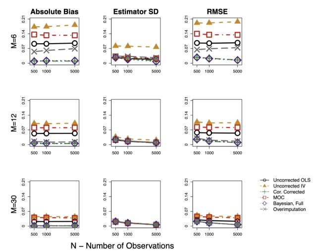
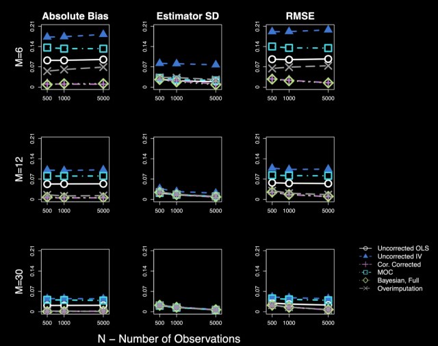
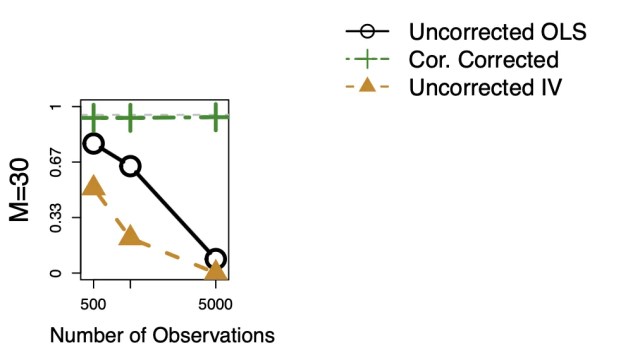
The paper combines simulations with several substantive applications to show when corrections matter and how big the differences can be. Overall, naive regressions almost always understate the strength of relationships involving latent predictors, MOC frequently makes that understatement worse, uncorrected IV overshoots, and the split‑indicator correction dramatically reduces bias.

Political knowledge predicting sense of duty to vote

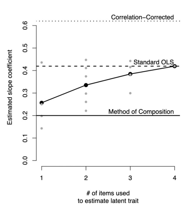
Using American National Election Study data, we estimate a latent political knowledge scale from four factual questions and regress a “duty to vote” scale on that latent predictor. A standard regression using the full four‑item knowledge score yields a slope of about 0.42, while the corrected estimator pushes that to about 0.62—almost a 50% increase in the estimated effect. By contrast, the method of composition cuts the slope down to roughly 0.20, and uncorrected IV more than doubles it, illustrating how both standard fixes misbehave in this setting.

Ideology predicting presidential vote choice

In a second example using the 2016 Cooperative Congressional Election Study, we estimate latent ideology from 30 policy items and use it to predict presidential vote choice. With such a rich set of indicators, the latent trait is measured relatively precisely, so the correction is modest but still detectable: naive slopes are attenuated, and the corrected estimator recovers a slope very close to the “true” value in simulations. When they intentionally restrict the number of items to mimic typical shorter scales, the correction grows, and naive OLS can underestimate slopes by 20–35%.

Democracy indices and economic growth

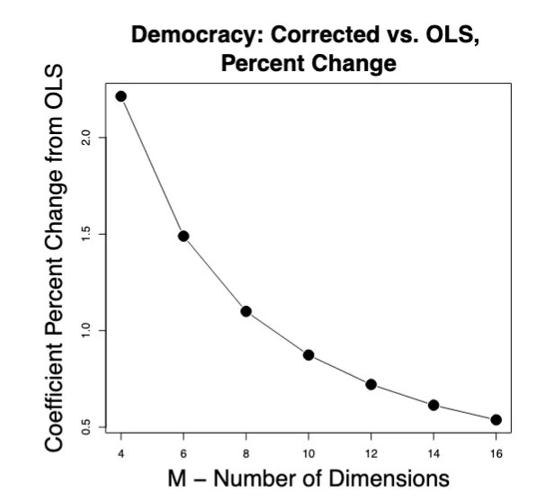
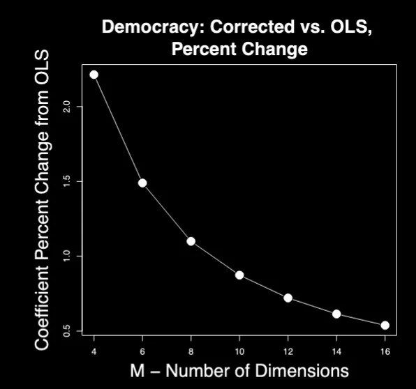
The paper revisits the relationship between democracy and economic growth using Freedom House sub‑indicators and a principal‑components democracy scale. Here, the indicators are highly correlated, and the latent democracy measure is relatively stable, so the split‑indicator correction barely moves the estimated effect. This example shows that the method can also reassure researchers when measurement error is small enough to be negligible.

Text‑based sentiment and incumbent vote share

Finally, we apply this approach to text data, using a pre‑trained language model to score the sentiment of U.S. House floor speeches, then relating sentiment to incumbent vote share. Because sentiment is a noisy latent construct built from long speeches and segment‑level predictions, the corrected estimates are about 14% larger in magnitude than the naive ones. This highlights how AI‑based text scores, which are increasingly common in political communication research, are also natural candidates for measurement‑error correction.

When should researchers worry about measurement error in latent predictors?

You do not always need a correction—but you should check. The paper provides guidance on when the split‑indicator method is likely to matter and when naive regression is probably fine.

• High‑stakes latent predictors: If the key independent variable is a latent trait (e.g., democracy, ideology, knowledge) central to your theory, you should almost always assess measurement error.
• Few indicators (small item batteries): When scales are built from only 3–10 items, attenuation can easily reach 20–50%.
• Text and ML scores: Embeddings, sentiment, and other model‑based scores are latent by design and often quite noisy.
• Control variables: Even if the latent predictor is “just” a control, mis‑measurement can bias other coefficients of interest.
• Highly correlated indicators and many items: In settings like roll‑call‑based legislator ideal points with hundreds of votes, measurement error is often small and corrections may be negligible.

How can I apply this correction method in my own research?

We provide open‑source software so applied researchers can easily implement the split‑indicator correction. The workflow is intentionally simple and designed to slot into existing data analysis pipelines.

1. Choose your indicators and estimation strategy. Decide which items measure your latent trait and how you will estimate it (e.g., additive index, factor model, IRT, ML model).
2. Partition indicators. Randomly split the indicators into two disjoint sets (as balanced as possible) and estimate the latent trait separately on each set to get \hat X_1 and \hat X_2.
3. Estimate the outcome model. Run naive OLS or IV using one split as the predictor, then apply the correlation‑based correction using \text{Cor}(\hat X_1, \hat X_2).
4. Average across partitions. Repeat for multiple random partitions and aggregate (for example, using the median across partitions) to stabilize results.
5. Use the provided software. Our package at GitHub.com/cjerzak/lpme-software implements these steps, including bootstrap uncertainty for both the slope and the correction factor.

Key takeaways for political scientists and other social scientists

This paper’s main message is that latent predictors are not just another noisy variable—they combine measurement error with identification choices in a way that breaks standard intuition about correction methods. If you plug latent scores into regressions without thinking about this, you are probably understating the strength of the relationships you care about.

• Latent predictors are almost always measured with error, and that error interacts with arbitrary scaling rules.
• Naive OLS tends to attenuate effects; the method of composition often makes that attenuation worse; standard IV overcorrects.
• A split‑indicator, correlation‑adjusted estimator can dramatically reduce bias while remaining easy to implement with existing measurement strategies.
• In real applications, corrected effects are often 10–50% larger than naive estimates, which can materially change substantive conclusions.
• Open‑source tools mean there is little excuse not to check how sensitive your results are to latent‑predictor measurement error.

FAQ: Measurement error in latent predictors

TL;DR: What is lpmec?

lpmec is an R package for latent predictor measurement error correction: when your key regressor is a latent score (ideology, knowledge, democracy, sentiment, etc.) estimated from indicators, naive regression slopes are typically attenuated toward zero. The package implements a split-indicator correction with bootstrap inference, and also supports Bayesian MCMC—including a joint Bayesian measurement-and-outcome model.

• Problem: latent predictors are noisy and identified on an arbitrary scale (e.g., mean 0, variance 1).
• Fix: split indicators into two halves, estimate the latent trait twice, and correct slopes using the cross-half correlation.
• Inference: bootstrap over resamples and multiple random splits/partitions.
• Bayesian options: MCMC via pscl (R) or NumPyro (Python/JAX), plus mcmc_joint.
• Speed: the NumPyro backend can leverage JAX JIT/XLA and optional GPU/TPU execution.

What does lpmec do?

The package provides tools to estimate regression effects when the key predictor is a latent trait inferred from multiple observed indicators. It focuses on the common applied workflow: estimate a latent score first, then regress an outcome on that score. When done naively, this “two-stage” approach typically understates effects because measurement error lives on the right-hand side.

lpmec implements split-sample IV and correlation-adjusted OLS/IV estimators that remain valid under latent-scale identification, and wraps the whole procedure in a bootstrap to deliver uncertainty quantification (standard errors and percentile confidence intervals). See the accompanying paper: Jerzak & Jessee (2025).

How does it work?

The core idea is to create two independent measurements of the same latent trait by splitting the indicators, then use their relationship to correct attenuation. At a high level:

1. Split indicators. Partition the indicator set into two disjoint halves.
2. Estimate the latent trait twice. Produce two standardized scores, \hat X_1 and \hat X_2.
3. Measure reliability. Compute \rho = \mathrm{Cor}(\hat X_1, \hat X_2).
4. Correct slopes. Use split-sample IV and/or correlation-adjusted OLS/IV scaling based on \rho.
5. Stabilize + infer. Repeat across many random partitions and bootstrap resamples; aggregate (e.g., median across partitions) and form CIs.

In the package, lpmec_onerun() performs a single partition run, while lpmec() orchestrates partitions + bootstrapping and returns the final estimates.

Estimation backends

You can plug in different measurement models for the latent trait while keeping the same correction machinery:

• EM IRT (default): binary/ordinal IRT via emIRT.
• PCA: first principal component of indicators.
• Averaging: simple additive index.
• MCMC: Bayesian IRT via pscl::ideal (R) or NumPyro (Python/JAX).
• Custom: provide your own latent estimation function.

Joint Bayesian model (and why)

Beyond modular “estimate-then-regress” corrections, lpmec supports mcmc_joint, a joint Bayesian measurement-and-outcome model that simultaneously estimates latent traits and the outcome relationship. Conceptually, it couples an IRT measurement model for indicators X_{ij} with an outcome model like Y_i \sim \mathcal{N}(\alpha + \beta \theta_i,\ \sigma), so posterior uncertainty in \theta_i propagates directly into inference on \beta.

This can be attractive when you want a fully probabilistic joint specification, at the cost of higher computational demands and stronger modeling assumptions.

GPU acceleration via JAX/NumPyro

When you choose the NumPyro backend (mcmc_control = list(backend = "numpyro")), sampling runs through JAX. JAX provides automatic differentiation and JIT/XLA compilation; with a CUDA-enabled jaxlib installation and a compatible GPU, the same model can execute on GPU/TPU. NumPyro also supports parallel (and in some settings vectorized) multi-chain execution, which can further improve throughput.

• Default is CPU-only: the package works without Python when using non-NumPyro methods.
• Optional acceleration: NumPyro/JAX can speed up HMC/NUTS, especially for larger item batteries or repeated runs.
• Practical tip: GPU use depends on your Python environment (installing the correct jaxlib build); once present, JAX selects the accelerator automatically.

How to use it

Source and documentation live here: GitHub.com/cjerzak/lpmec-software.

Minimal R usage

library(lpmec)
data(KnowledgeVoteDuty)
res <- lpmec(
  Y = KnowledgeVoteDuty$voteduty,
  observables = as.matrix(KnowledgeVoteDuty[, 2:5]),
  n_boot = 50L,
  n_partition = 10L,
  estimation_method = "em"
)
summary(res)

Optional: NumPyro backend (enables JAX; GPU if configured)

library(lpmec)
build_backend()  # creates conda env + installs jax/numpyro
res_joint <- lpmec(
  Y = Yobs,
  observables = ObservablesMat,
  n_boot = 0L,
  n_partition = 1L,
  estimation_method = "mcmc_joint",
  mcmc_control = list(backend = "numpyro", n_chains = 2L),
  conda_env = "lpmec"
)

Key takeaways

• lpmec targets attenuation bias caused by noisy latent predictors under identification constraints.
• It is modular: you can use EM IRT, PCA, simple indices, MCMC, or custom latent estimators.
• lpmec() provides bootstrap uncertainty and aggregates over many indicator splits.
• mcmc_joint offers a fully joint Bayesian alternative when you want end-to-end probabilistic modeling.
• NumPyro/JAX provides a clear path to GPU acceleration for computationally heavy MCMC workflows.

FAQ