
Authors: Connor Jerzak | Ritwik Vashistha | Adel Daoud
TL;DR
This paper shows how Earth observation (EO) satellite image sequences can act like “context sensors” for randomized controlled trials (RCTs), helping estimate heterogeneous treatment effects (CATEs) and transport experimental evidence to new places. Across three real-world RCTs (Georgia, Peru, Uganda), image-sequence-based approaches often rival or outperform traditional tabular covariate methods while being globally scalable and historically available.
- What’s new: Use time series satellite imagery (not just a single snapshot) as pre-treatment context for CATE discovery and generalization.
- How it’s done: Extract compact embeddings with computer vision (random, pre-trained, EO-trained foundation models) and plug them into causal heterogeneity models; evaluate with RATE (Rank-Weighted ATE).
- Why it matters: Surveys and admin covariates can be expensive, missing, and hard to extend beyond the study site; satellite imagery is broadly available and repeatable over time.
What problem does the paper solve?
Traditional heterogeneity analysis leans on survey or administrative “tabular” data, which can be costly to collect and may only exist inside the original trial footprint. The paper proposes a scalable alternative: use pre-treatment satellite imagery—especially image sequences—to represent local context (built environment, land use, infrastructure, environmental conditions) and feed those representations into modern causal inference tools.
Big idea: Treat satellites as “contextual sensors” for experiments—capturing time-varying, location-specific information you can reuse for both heterogeneity and generalization.
What are ATE and CATE (in plain English)?
The ATE is the average effect of treatment across everyone; the CATE is the effect for a subgroup defined by features like demographics—or here, satellite-derived representations of place and history.
In the paper’s notation:
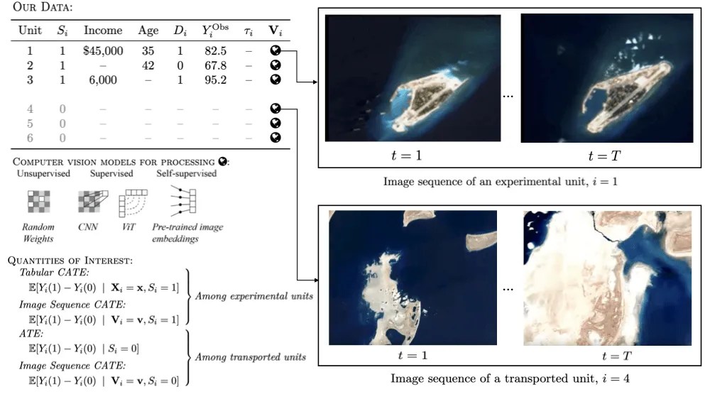
\text{ATE}=\mathbb{E}[Y(1)-Y(0)]\quad\text{and}\quad \tau(x)=\mathbb{E}[Y(1)-Y(0)\mid X=x]They also define “image CATEs” and “video (sequence) CATEs” by conditioning on satellite imagery:
\tau(m)=\mathbb{E}[Y(1)-Y(0)\mid M=m],\quad \tau(v)=\mathbb{E}[Y(1)-Y(0)\mid V=v]- ATE answers: “Does the program work on average?”
- CATE answers: “Where / for whom does it work best (or backfire)?”
Why satellite image sequences (not single images)?
A single image is a snapshot; a sequence captures trajectories—how places evolve pre-treatment—which may better explain why treatment effects differ across locations.
The paper argues that the temporal dimension can reveal context that cross-sectional measures miss, especially when development patterns or environmental change shape responsiveness to policy. Practically, sequences are created by extracting pre-treatment images over time (e.g., multi-year composites) for each experimental unit’s coordinates.
Satellite sequences are powerful when: infrastructure, land use, urbanization, or environmental conditions change over time in ways that plausibly moderate the intervention’s effect.
How does the EO-to-CATE pipeline work?
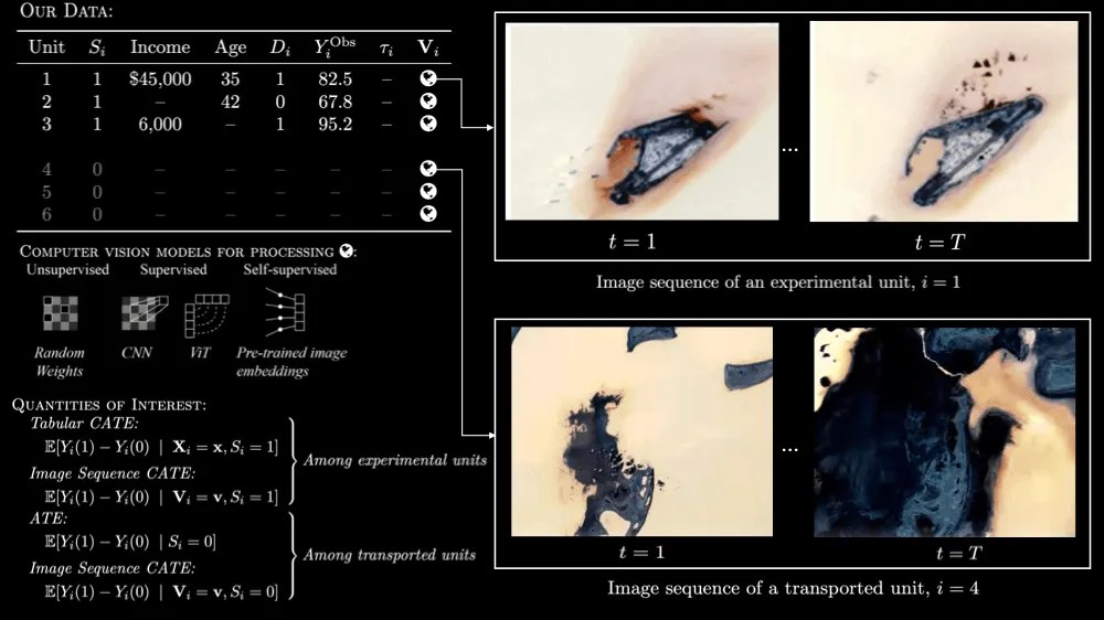
Geocode units → pull pre-treatment satellite image sequences → encode them into compact embeddings with computer vision → estimate CATEs with causal ML → validate heterogeneity using RATE → (optionally) transport effects to new locations.
- Index experimental units to coordinates. (Households, villages, census blocks, etc.)
- Extract pre-treatment EO imagery. Build a chronological sequence for each unit.
- Represent images with computer vision. Use random projections, pre-trained models, or EO-trained foundation models to get low-dimensional vectors.
- Estimate heterogeneous effects. Feed embeddings into a heterogeneity model (e.g., causal forests / R-learner families).
- Evaluate whether heterogeneity is real. Use RATE / RATE ratio to test whether the ranking rule meaningfully prioritizes high responders.
- Transport to new places. Embed non-experimental locations and predict transported effects with overlap diagnostics.
What computer vision models do they compare?
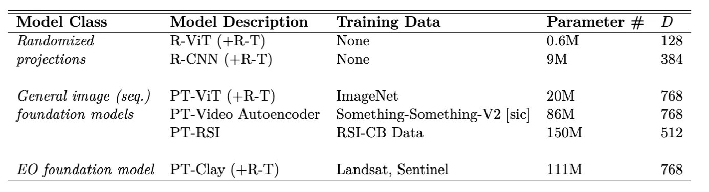
They compare (1) randomized projections, (2) non-EO pre-trained vision models, and (3) EO-trained models—because domain-specific pretraining can encode patterns that matter for Earth observation tasks.
Here’s the paper’s high-level model menu (summarized from its model table):
| Model class | Examples | Why it matters |
|---|---|---|
| Randomized projections | Randomized Vision Transformer | Fast, no training data needed; can preserve useful geometry. |
| Pre-trained (non-EO) | ViT (ImageNet), Swin (ImageNet-1K), Video Autoencoder | Strong generic visual features; may miss EO-specific semantics. |
| EO-trained | Clay (Landsat/Sentinel), CLIP-RSICD | Encodes EO-relevant signals (e.g., land use, vegetation, urbanization). |
Why this comparison is useful: It helps practitioners choose between “no-data” baselines, general-purpose vision backbones, and specialized EO foundation models depending on budget, compute, and task fit.
How do they evaluate heterogeneity if CATEs are unobserved?
They use RATE (Rank-Weighted Average Treatment Effect), which tests whether a model’s prioritization rule actually identifies units with above-average treatment effects when you “treat the top-ranked first.”
The core idea: produce a score S(V) that ranks units by predicted benefit; then check whether the observed experimental outcomes imply higher effects among the top-ranked subsets. The paper writes RATE as:
\text{RATE}=\int_0^1 \alpha(q)\Big(\mathbb{E}[Y(1)-Y(0)\mid F(S(V))\ge 1-q]-\mathbb{E}[Y(1)-Y(0)]\Big)\,dqThey also report a RATE ratio (estimate divided by its standard error) as a simple “is there detectable heterogeneity?” diagnostic.
What are the three RCT case studies?
1) Georgia (USA): Water conservation messaging
Key details: A large RCT in Cobb County, Georgia (2007) with household water consumption outcomes; EO sequences built from Landsat 5 composites over ~10 years pre-treatment.
2) Peru: Graduation program outcomes
Key details: A multifaceted program (around 2011) with an asset index outcome; EO sequences from Landsat 5 built as multi-year median composites going back to 2001.
3) Uganda: Grants for entrepreneurship
Key details: A grant-based anti-poverty intervention (2008); due to limited imagery availability, analysis uses a single-image approach (decadal mosaic) rather than sequences.
What did they find (key results)?
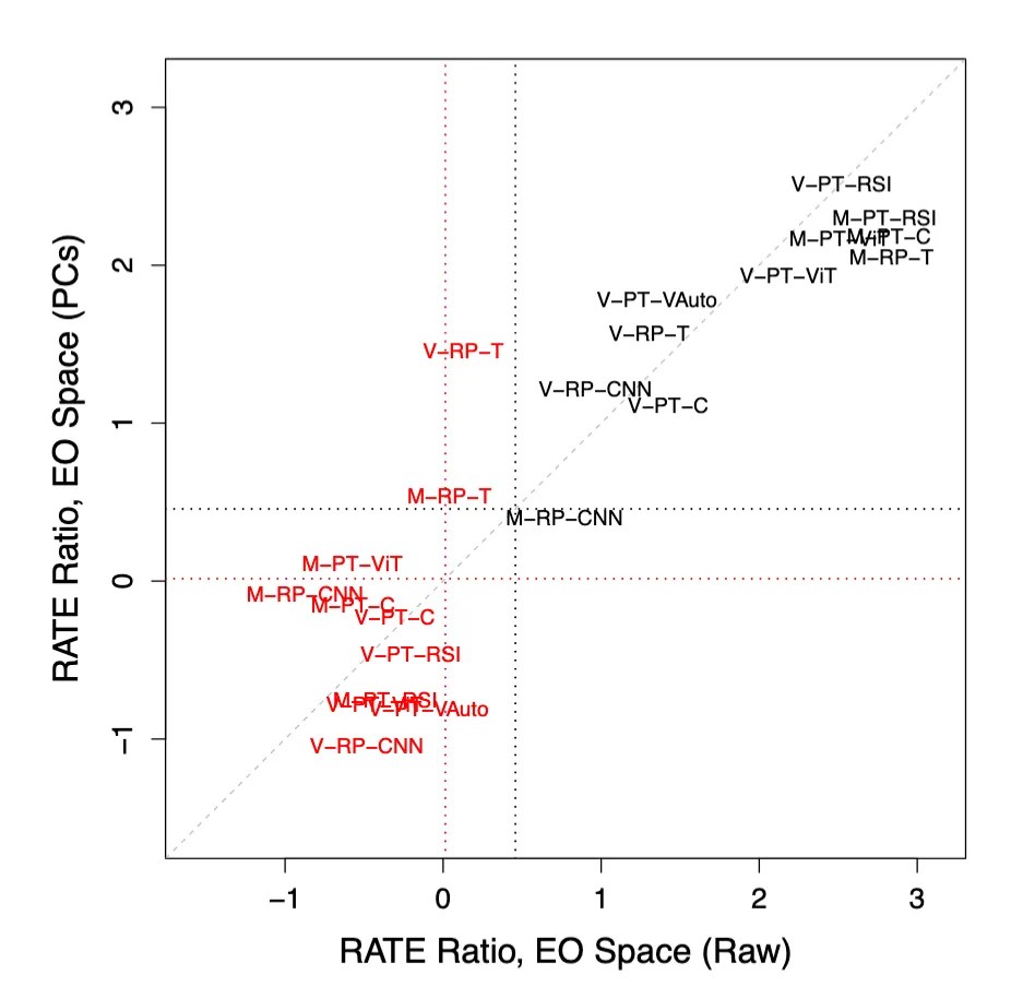
Across settings, EO image-sequence features frequently deliver heterogeneity signals that match or beat tabular baselines, and EO-trained models plus temporal sequences tend to improve detection.
- EO-only can be competitive: In multiple configurations, satellite-derived representations rival tabular covariates for heterogeneity discovery.
- Sequences help: Moving from single images to image sequences often strengthens the heterogeneity signal (consistent with the paper’s multivariate summary).
- EO pretraining helps: EO-fine-tuned foundation models tend to outperform random projections and non-EO pretraining when extracting useful context.
- Dimensionality reduction isn’t free: Compressing embeddings too aggressively (e.g., PCA) can weaken heterogeneity signals in some cases.
Practical takeaway: If you can afford the data pull and embeddings, start with an EO-trained model and a short pre-treatment time series—then validate with RATE before trusting subgroup stories.
How does “transportability” work here?
They estimate “transported” effects by predicting treatment effects for non-experimental locations based on how similar their EO embeddings are to places in the original trial—then add an overlap diagnostic to flag extrapolation risk.
The transported estimand is expressed as:
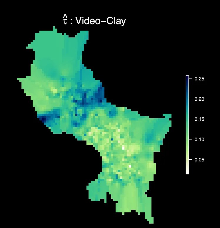
\tau_{\text{transport}}(v)=\mathbb{E}[Y(1)-Y(0)\mid V=v,\;S=0]Operationally, the paper samples new points (e.g., additional census blocks / population-weighted locations), builds EO embeddings, predicts effects, and visualizes transported effect maps—with an “overlap” view based on nearest-neighbor distances in embedding space.
Satellite imagery vs tabular covariates: when should you use what?
Use satellite imagery when you need scalable, consistent context (especially beyond your sample); use tabular covariates when you need direct individual attributes and have reliable coverage—ideally combine both when feasible.
Satellite imagery is best when you need:
- Scalability: apply the same covariate pipeline across regions and years
- Historical context: pre-treatment trajectories and environmental change
- Transportability: extend predictions to places without survey coverage
Tabular covariates are best when you need:
- Individual-level traits not visible from space (e.g., education, attitudes)
- Mechanism tests using socio-demographic detail
- Local nuance satellites may proxy imperfectly
Best of both: Combine EO embeddings + tabular data when your goal is maximum predictive signal and interpretability—then test for incremental value (e.g., higher RATE ratios, stability in subgroup rankings).
Limitations and next steps
Transporting effects relies on assumptions (model correctness, limited spillovers), and the approach needs careful validation for uncertainty, extrapolation, and robustness before policy deployment.
- Robustness: transported maps may be sensitive to representation/model choices.
- Spillovers: large-scale policies can create spillovers that complicate CATE interpretation.
- Uncertainty: deep EO models make uncertainty quantification non-trivial.
- Site selection bias: where RCTs are run may not represent where you want to generalize.
FAQ
What is Earth observation (EO) data?
EO data is satellite (or aerial) imagery that measures features of Earth’s surface over time. In this paper, EO images provide scalable, pre-treatment context for each experimental unit.
Do I need “big data” to use this approach?
Not necessarily—because you can use pre-trained or EO-trained models as feature extractors without training a deep vision model from scratch. The key is having geolocated units and access to suitable imagery.
Why not just use land cover maps instead of raw imagery?
Land cover maps are useful but compress information into fixed categories and may be updated infrequently. Raw imagery (especially sequences) can preserve richer signals that sometimes yield stronger heterogeneity detection.
What does RATE tell me that a correlation doesn’t?
Correlation compares two sets of predicted effects, but it doesn’t test whether your prioritization actually improves outcomes. RATE directly evaluates whether ranking units by predicted benefit identifies subgroups with higher observed treatment effects.
Can this help decide where to scale a policy?
Potentially—transported effect maps can highlight where impacts might be larger or smaller, and overlap diagnostics can flag where predictions are more extrapolative. You still need strong validation and policy-specific safeguards.
Where can I find the implementation?
The authors provide open-source code at AIandGlobalDevelopmentLab/causalimages-software.
Conclusion
If your RCT is geolocated, satellite image sequences can help unlock scalable heterogeneity analysis and more credible generalization—without depending entirely on expensive, site-bound covariates.
If you’re building evidence pipelines that need to “travel” across districts, states, or countries, this paper is a strong reference point: it shows a concrete, testable workflow that connects EO foundation models with causal inference—plus a practical validation metric (RATE) and a transportability map pattern for decision support.


–
References
@article{jerzak2024effect,
  title={Effect Heterogeneity with Earth Observation in Randomized Controlled Trials: Exploring the Role of Data, Model, and Evaluation Metric Choice},
  author={Jerzak, Connor T. and Ritwik Vashistha and Adel Daoud},
  journal={ArXiv Preprint},
  year={2024},
  volume={},
  pages={},
  publisher={}
}
–
Related Work
@article{fucheng2025optimizing,
  title={Optimizing Multi-Scale Representations to Detect Effect Heterogeneity Using Earth Observation and Computer Vision: Applications to Two Anti-Poverty RCTs},
  author={Fucheng, Warren Zhu and Connor T. Jerzak and Adel Daoud},
  journal={Proceedings of the Fourth Conference on Causal Learning and Reasoning (CLeaR), Proceedings of Machine Learning Research (PMLR)},
  year={2025},
  volume={},
  pages={},
  publisher={}
}[Video][>]
–
@article{daoud2026chinese,
  title={Chinese vs. World Bank Development Projects: Insights from Earth Observation and Computer Vision on Wealth Gains in Africa, 2002-2013},
  author={Daoud, Adel and Cindy Conlin and Connor T. Jerzak},
  journal={World Development},
  year={2026},
  volume={202},
  pages={107328},
  publisher={}
}–
@article{jerzak2023image,
  title={Image-based Treatment Effect Heterogeneity},
  author={Jerzak, Connor T. and Fredrik Johansson and Adel Daoud},
  journal={Proceedings of the Second Conference on Causal Learning and Reasoning (CLeaR), Proceedings of Machine Learning Research (PMLR)},
  year={2023},
  volume={213},
  pages={531-552},
  publisher={}
}–
@article{sakamoto2024scoping,
  title={A Scoping Review of Earth Observation and Machine Learning for Causal Inference: Implications for the Geography of Poverty},
  author={Sakamoto, Kazuki and Connor T. Jerzak and Adel Daoud},
  journal={To appear in: Hall, Ola and Ibrahim Wahab (eds.), Geography of Poverty},
  year={2024},
  volume={},
  pages={},
  publisher={Edward Elgar Publishing (Cheltenham, UK)}
}–
@article{jerzak2023integrating,
  title={Integrating Earth Observation Data into Causal Inference: Challenges and Opportunities},
  author={Jerzak, Connor T. and Fredrik Johansson and Adel Daoud},
  journal={ArXiv Preprint},
  year={2023},
  volume={},
  pages={},
  publisher={}
}–
@article{jerzak2023causalimages,
  title={CausalImages: An R Package for Causal Inference with Earth Observation, Bio-medical, and Social Science Images},
  author={Jerzak, Connor T. and Adel Daoud},
  journal={ArXiv Preprint},
  year={2023},
  volume={},
  pages={},
  publisher={}
}–