
Authors: Connor Jerzak | Rebecca Goldstein | Aniket Kamat | Fucheng Warren Zhu
TL;DR: Rerandomization improves power in randomized experiments by discarding treatment assignments with poor covariate balance, but in high-dimensional designs it can be painfully slow. The fastrerandomize R package combines JAX, batched kernels, GPU/TPU support, and memory-efficient key-only storage to make rerandomization in R practical even with thousands of units and covariates, while still supporting design-respecting randomization tests and power diagnostics.
What problem does rerandomization actually solve in experiments?
Rerandomization in experimental design attacks a familiar headache: covariate imbalance between treatment and control groups. Instead of accepting the first random assignment, you repeatedly rerandomize until a balance rule is satisfied, which reduces variance and makes treatment effect estimates more precise.
Even with perfect randomization, you can get unlucky draws. Imagine an experiment with 50 villages where the coin flip sends almost all high-poverty villages to treatment and low-poverty villages to control. The design is technically valid, but estimates will be noisy and controversial because key covariates are badly imbalanced.
Rerandomization experimental design turns this into a simple loop:
- Draw a random assignment (e.g., 25 treated, 25 control).
- Compute a balance metric (like Mahalanobis distance or Hotelling’s T²) on pre-treatment covariates.
- Accept the assignment only if the covariate balance is “good enough,” otherwise rerandomize and try again.
This keeps the core benefit of randomization (no cherry-picking based on outcomes) but conditions on assignments that achieve better covariate balance in the variables you believe are prognostic. In the fastrerandomize paper, the authors formalize this workflow and show how to run GPU accelerated rerandomization in R so it remains feasible even when each unit has hundreds or thousands of covariates.
From a power perspective, rerandomization reduces the portion of variance driven by covariate imbalance while leaving the irreducible noise alone. That means tighter confidence intervals, more stable estimates, and a lower chance that your main result hinges on a single unlucky random split of the sample.
When is rerandomization worth it — and when is it overkill?
Rerandomization pays off the most when your covariates are genuinely predictive of the outcome (high R²) and you are not in an extremely massive, low-signal regime. If covariates are weak or your sample size is enormous, aggressive rerandomization can burn compute without giving you meaningful gains over complete randomization.
The key intuition from the paper is that covariate imbalance adds a second variance term on top of residual noise. Under a simple linear model, the RMSE of a difference-in-means estimator can be decomposed into:
- a “noise term” driven by unexplained outcome variance, and
- a “design term” driven by how aligned your covariate imbalance is with the true prognostic direction.
Rerandomization shrinks that design term. How much that matters depends heavily on R², the share of outcome variance explained by covariates:
- High R² (e.g., 0.4–0.6): imbalance hurts you a lot, so rerandomization can noticeably reduce RMSE and improve power.
- Low R² (e.g., < 0.1): covariates barely predict the outcome, so balance has little impact on precision.
The fastrerandomize diagnostics in the paper show this numerically. For a design with 500 treated and 500 control units and R² = 0.5, keeping only the best 1% of assignments by a multivariate balance metric can reduce RMSE by roughly 15% in a 30-dimensional covariate set but only about 3% in a 1000-dimensional set. In high-dimensional experimental design, you often need more stringent rerandomization (smaller acceptance probabilities) to get the same precision boost.
Practical rules of thumb:
- Rerandomize if an unlucky imbalance plot would trouble you. If you would be uncomfortable publishing a histogram where treatment and control differ sharply on key pre-treatment variables, rerandomization is cheap insurance.
- The more expensive the experiment, the more rerandomization is worth the compute. If each unit costs real money or time (field trials, clinical experiments, lab work), spending GPU hours to improve covariate balance is almost always a good trade.
- For huge online A/B tests with weak covariates, complete randomization may be fine. When n is in the millions and your pre-exposure variables are noisy, small improvements in covariate balance rarely change decisions.
So if your design relies on rich pre-treatment features that truly help predict outcomes, rerandomization in R is a high-leverage knob. If your covariates are mostly noise, focus on sample size, measurement, and analysis instead.
How does rerandomization compare to blocking, matching, and regression adjustment?
Rerandomization complements blocking, matching, and regression adjustment; it does not replace them. Blocking and matching structure the design before randomization, regression soaks up remaining imbalance after the fact, and rerandomization directly constrains the randomization itself to enforce covariate balance.
Here is a quick comparison of these tools in the context of covariate balance in randomized experiments:
| Method | When it acts | How it works | Strengths | Limitations |
|---|---|---|---|---|
| Blocking | Design stage | Form discrete strata (e.g., by site, gender, baseline risk) and randomize within each block. | Simple, interpretable, especially strong for a few key categorical covariates. | Hard to scale to many or continuous covariates; block explosion in high dimensions. |
| Matching | Design stage | Pair or group similar units (e.g., via propensity scores) and randomize within matches. | Fine-grained control when covariates are low- to moderate-dimensional. | Can struggle and become brittle in very high-dimensional feature spaces. |
| Rerandomization | Design stage | Draw many assignments, keep only those with good balance according to a metric like Hotelling’s T². | Works naturally with continuous, high-dimensional covariates and a single scalar balance metric. | Naive implementations are slow; requires explicit acceptance rule and careful computation. |
| Regression adjustment | Analysis stage | Regress outcomes on treatment and covariates to reduce residual variance. | Easy to add to almost any analysis; powerful when models are well-specified. | Does not fix poor design; can be sensitive to model misspecification. |
If you think in “X vs Y” terms:
- Rerandomization vs blocking: blocking is great for a few discrete strata; rerandomization shines when you care about multivariate balance on many continuous features.
- Rerandomization vs matching: matching pairs units first, then randomizes; rerandomization keeps the simple complete-randomization structure but rejects bad draws based on a balance metric.
- Rerandomization vs regression: regression without rerandomization leaves power on the table if covariates are very prognostic, while rerandomization without regression wastes information about the functional form of the outcome model. Together, they are often best.
The fastrerandomize R package assumes you may still block or match on a few key variables, then rerandomize within that design using a high-dimensional balance metric such as Hotelling’s T². Regression adjustment can then further clean up any residual imbalance when you estimate effects.
Why is rerandomization usually slow — and how does fastrerandomize make it fast?
Naive rerandomization in R loops over candidate assignments on the CPU, computes balance statistics one at a time, and often stores full assignment matrices. As the number of units and covariates grows, this approach blows up in both runtime and memory.
The fastrerandomize R package solves this with three main ideas: batched balance checks, GPU/TPU acceleration, and key-only storage. Under the hood, it uses JAX and XLA to compile vectorized kernels that evaluate thousands of candidate assignments in parallel, and it stores only the random-number keys for accepted draws rather than full 0/1 assignment vectors.
The architecture is two-layered:
- An R front-end that exposes a compact API for building backends, generating randomizations, diagnosing stringency, and running randomization tests in R.
- A JAX backend (via reticulate) that compiles batched candidate generation, balance evaluation, and inference kernels and dispatches them to CPU, GPU, or TPU via XLA.
Batched balance checks mean you amortize overhead across large blocks of candidates. Instead of computing a Mahalanobis or Hotelling’s T² distance for one assignment at a time, fastrerandomize evaluates thousands of assignments in a single linear algebra call, which maps perfectly to GPUs.
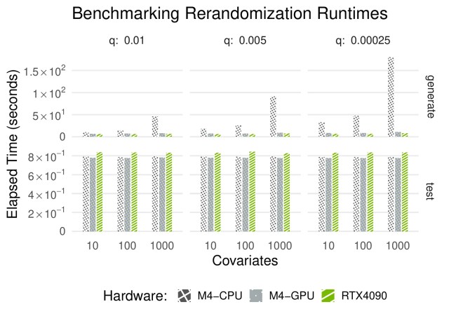
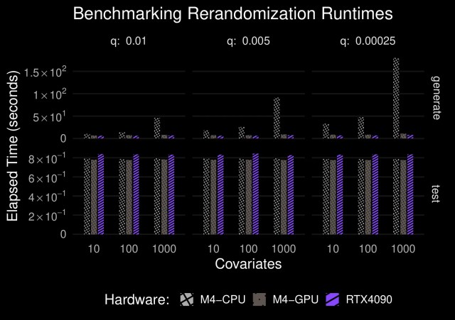
Hardware acceleration exploits modern compute. On laptops with Apple’s METAL backend or machines with GPUs, the same JAX code can run orders of magnitude faster than pure R implementations, especially when the acceptance probability is small and you need huge candidate pools in high-dimensional designs.
Key-only storage keeps memory usage under control. Instead of storing every accepted assignment as an n-length binary vector, fastrerandomize stores the PRNG keys that generate those assignments. When you need a particular assignment—for plotting, exporting, or inference—the key is replayed to regenerate it. If n is 1000 and each key is just a couple of integers, this can mean hundreds of times less memory than storing full matrices.
In benchmarks, this approach delivers order-of-magnitude speedups over baseline R rerandomization workflows as both the sample size and covariate dimension increase, making GPU accelerated rerandomization a practical default instead of a theoretical ideal.
How do you choose a rerandomization acceptance probability (q) in practice?
The acceptance probability q controls how strict your balance rule is: smaller q means you keep only the best-balanced assignments, but you need larger candidate pools to find them. In fastrerandomize, you specify q directly and can use the diagnose_rerandomization() function to connect that choice to expected RMSE reduction and power.
Conceptually, rerandomization “keeps the best q%” of candidate assignments according to a multivariate balance metric such as Hotelling’s T². If q = 0.01, you are keeping roughly the best 1% of assignments, which typically means you need about 1/q ≈ 100 draws per accepted assignment on average.
The paper shows that this interacts strongly with dimension. At acceptance probability q = 0.01:
- In a 30-dimensional design, rerandomization shrinks the imbalance-driven variance term substantially and can reduce RMSE by around 15% relative to complete randomization.
- In a 1000-dimensional design, the same q = 0.01 only shrinks the imbalance term modestly and yields about a 3% RMSE reduction.
In other words, as dimension grows, you need more aggressive rerandomization to keep the same level of balance. In a high-dimensional example with 1000 covariates, 500 treated and 500 control units, R² ≈ 0.4, and a target effect size of about 0.2 standard deviations, the recommended acceptance probability that hits 80% power at 5% size is on the order of q* ≈ 0.000012—about eighty thousand candidate assignments per accepted one.
diagnose_rerandomization() automates this reasoning. You give it:
- design parameters: n_treated, n_control, d,
- an outcome scale and signal strength: R2 and a target effect size tau, and
- your desired size and power.
It then returns quantities like:
- the implied RMSE under complete randomization,
- the expected RMSE under a candidate acceptance probability q, and
- a recommended q* that meets your power target without wasting compute.
Practically, you can start with a coarse q (say 1%), check what the diagnostics say about RMSE and power, and then tighten q only if you need the extra precision. The “compute-precision frontier” visual in the paper makes this trade-off explicit: low-d designs get big gains with modest candidate pools; high-d designs require more selective rerandomization and thus larger candidate pools.
What does a full fastrerandomize workflow in R look like?
A typical fastrerandomize workflow in R has four steps: prepare covariates, choose an acceptance probability q, generate acceptable assignments (optionally on GPU), and run a design-respecting randomization test. The API is intentionally small: build_backend(), generate_randomizations(), diagnose_rerandomization(), and randomization_test() cover most use cases.
Here is a minimal, high-dimensional example that illustrates GPU accelerated rerandomization in R:
library(fastrerandomize)

# 1. Prepare covariates
set.seed(123)
X <- scale(matrix(rnorm(1000 * 200), nrow = 1000))  # 1000 units, 200 covariates

# 2. Choose stringency (e.g., keep best assignments by balance)
diag_out <- diagnose_rerandomization(
  n_treated = 500,
  n_control = 500,
  d         = ncol(X),
  R2        = 0.4,
  tau       = 0.2
)
q_star <- diag_out$recommended_q

# 3. Generate randomizations (GPU if available)
rand_obj <- generate_randomizations(
  n_units                   = nrow(X),
  n_treated                 = 500,
  X                         = X,
  randomization_type        = "monte_carlo",
  randomization_accept_prob = q_star
)

# 4. Run design-respecting randomization test
obsW <- rand_obj$randomizations[1, ]
obsY <- rnorm(nrow(X))  # replace with real outcomes

test_out <- randomization_test(
  obsW                     = obsW,
  obsY                     = obsY,
  candidate_randomizations = rand_obj$randomizations
)
Step 1 builds and scales your covariate matrix X; in high-dimensional experiments this might come from ML-derived features like embeddings from text, images, or networks. Step 2 calls diagnose_rerandomization() to find a rerandomization acceptance probability that hits your desired power target given your design and covariate predictiveness.
Step 3 calls generate_randomizations() with randomization_type = “monte_carlo”, which uses batched kernels and key-only storage to generate a large pool of acceptable assignments. If a GPU is available, the JAX backend will offload balance checks to accelerated hardware automatically.
Step 4 uses randomization_test() to carry out a design-respecting randomization test in R. You provide the observed assignment, outcome vector, and the candidate randomizations, and the function returns a randomization-based p-value and (optionally) a fiducial interval for your treatment effect.
This workflow is best for experiments where each unit has many pre-treatment features—say hundreds of ML-derived covariates—and you care about using rerandomization in R to achieve tight balance without hand-rolling custom GPU code.
How can you interpret randomization-based p-values and intervals from fastrerandomize?
fastrerandomize computes design-respecting randomization tests conditional on your rerandomization rule, so the reference distribution is built only from assignments that pass your balance criterion. This yields exact (or Monte Carlo) p-values for the sharp null and optional intervals that reflect the design you actually used, not an idealized complete randomization.
Standard asymptotic t-tests implicitly assume complete randomization or super-population models and ignore any acceptance rule you used during design. In contrast, rerandomization changes the distribution of your test statistic by excluding poorly balanced assignments, so good practice is to condition on that fact. Randomization tests in R implemented via randomization_test() do exactly this.
In practice:
- You choose a test statistic (often the difference-in-means or a regression-adjusted estimate).
- You compute that statistic on your observed assignment and on each accepted assignment in your candidate pool.
- Your randomization p-value is the fraction of accepted assignments whose statistic is as or more extreme than the observed one.
The minimum attainable p-value is 1 divided by the number of accepted assignments, because the smallest nonzero fraction you can get is “one extreme assignment out of M.” For example, with 1000 accepted assignments the smallest possible p-value is about 0.001; with 2000 accepted assignments, about 0.0005.
By inverting these design-respecting tests, fastrerandomize can also produce fiducial intervals for the effect of interest: you find the set of effect sizes that would not be rejected by a randomization test at your chosen alpha level. This kind of inference is especially appealing when you want your conclusions to rest on the actual rerandomization experimental design rather than large-sample approximations.
Should you use fastrerandomize for your next experiment?
You should use fastrerandomize when you care about tight covariate balance on truly prognostic features, especially in high-dimensional experiments where naive rerandomization in R would be too slow or memory-hungry. If your covariates are weak or your sample is enormous, simpler designs may already be close to optimal, but when imbalance threatens power, GPU accelerated rerandomization gives you a principled way to fix it.
A quick checklist:
- You have good pre-treatment covariates. Rerandomization is most valuable when covariates explain a substantial share of outcome variance (moderate to high R²).
- You can access a GPU or at least a solid CPU. The JAX backend makes it easy to tap into accelerated computing, but even CPU-only batched kernels can be a big step up from naive loops.
- You want design-based, not just model-based, inference. Randomization tests in R that respect your acceptance rule can feel more honest than relying solely on regression p-values.
- Your design is high-dimensional. If each unit is summarized by hundreds of features from text, images, or other ML pipelines, rerandomization experimental design with Hotelling’s T² is a natural fit.
To dive deeper:
- Read the full paper, “fastrerandomize: Fast Rerandomization Using Accelerated Computing”, for the full theory and benchmarks.
- Explore the source code and examples at the fastrerandomize R package repository.
- Try the interactive capsule at fastrerandomize.github.io/space to experiment with rerandomization acceptance probabilities and power diagnostics in your browser.
As LLMs and representation learning make high-dimensional covariates more common, tools like fastrerandomize will be increasingly important for bridging modern ML feature engineering with rigorous experimental design.
FAQ
What is rerandomization in experimental design?
Rerandomization in experimental design is the practice of repeatedly drawing treatment assignments until covariates are well balanced between treatment and control groups according to a pre-specified metric. It preserves the core benefits of randomization while reducing variance that comes from unlucky covariate imbalance.
Does rerandomization always improve power?
Rerandomization improves power when your pre-treatment covariates are genuinely prognostic for the outcome, because it reduces the variance associated with their imbalance. When covariates have little predictive value or sample sizes are enormous, the gains over complete randomization can be small relative to the extra computation required.
How is fastrerandomize different from other R randomization packages?
fastrerandomize is focused specifically on scalable rerandomization in R, combining batched balance checks, GPU/TPU acceleration, and key-only storage to handle very high-dimensional experiments and tight acceptance probabilities. It also builds in design-respecting randomization tests and diagnostics that link acceptance probability choices directly to expected RMSE and power.
Can I use fastrerandomize without a GPU?
Yes. The package uses JAX to target CPUs by default, so you can benefit from vectorized, compiled kernels even on a CPU-only machine. A GPU or TPU provides additional speedups, but is not required to run rerandomization in R with fastrerandomize.
For more: fastrerandomize.github.io and github.com/cjerzak/fastrerandomize-software
Performance: n = 100


Performance: n = 1000

References
@article{jerzak2026fastrerandomize,
  title={FastRerandomize: Fast Rerandomization Using Accelerated Computing},
  author={Jerzak, Connor T. and Rebecca Goldstein and Aniket Kamat and Fucheng Warren Zhu},
  journal={SoftwareX},
  year={2026},
  volume={33},
  pages={102508},
  publisher={}
}–
Related Work
@article{jerzak2023degrees,
  title={Degrees of Randomness in Rerandomization Procedures},
  author={Jerzak, Connor T. and Rebecca Goldstein},
  journal={ArXiv Preprint},
  year={2023},
  volume={},
  pages={},
  publisher={}
}
–